Abstract
This paper presents the results of a numerical study on airflow modeling in a room with mixing ventilation. Results which are based on the mean age of air (MMA) are validated against existing experimental works in the literature. The numerical results were obtained by performing CFD analysis using the AirDummies software while the tracer gas concentration decay method is employed for experimental measurements. k-ω SST turbulence model is used along with proper boundary conditions to find the velocity field and MMA. The inlet velocity of 1.68 m/s and air changes per hour (ACH) of 8 were set with Schmidt number of 2 for MMA diffusion modeling. The room modeled was 4.2 m long, 3.6 m wide, and 3 m high which is exactly similar to the dimensions used in the experimental work. The MMA was calculated at different heights at the distance of 1.13 m, 2.2 m, 3.2 m from the west-facing wall. It is shown that AirDummies provides pretty much the same results as the experimental work.
Introduction
Over the last decade, the significance of indoor air quality (IQA) has increased considerably, as individuals tend to spend a significant amount of their time indoors. A key parameter used to assess IQA is the mean age of air (MAA), which is the average time that the air circulates inside a building before it is replaced by fresh outdoor air. Although the tracer gas method is the usual technique used to determine MAA, it is time-consuming and costly. However, computational fluid dynamics (CFD) provides an alternative solution to analyze MAA values in a building. This paper aims to demonstrate the capability of AirDummies software in calculating MAA in buildings.
Experimental Setup
The MMA measurements were conducted in a test room of size (4.2, 3.6, 3) meters (length, width, height) with isothermal mixing ventilation (see Figure 1) [1]. The inlet air supply with dimensions of 0.3 m × 0.2 m was located in the middle of the west wall where the lower edge was placed 2.05 m above the ground level. It is indeed an important task to make sure the inlet velocity profile is as uniform as possible; in order to achieve such goal, a special lemniscate-shaped inlet nozzle was employed. On the other hand, the outlet was set on the ceiling, closer to the east wall and on the other side of the room opposite to the air inlet. In order to minimize the temperature effects, the room under study was placed in another enclosure with the exact same temperature. The average inlet air velocity was 1.68 m/s with ±0.03 m/s fluctuations. The ventilation rate was approximately 363 𝑚3/ℎ𝑟, i.e., which yields ACH of 8. It is worth mentioning that the temperature was kept constant at 23±0.3 °C.
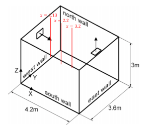
Figure 1: Schematic of the test room with the location of MAA measurements
As mentioned earlier, the main goal of this paper is to validate the CFD employed by AirDummies against the experimental data using MAA. Therefore, it is vital to perform the MAA measurements delicately and with extra care. The concentration decay method was employed to evaluate the MAA using SF6 as the tracer gas. At first, the room was set with no ventilation so that the tracer gas reaches a uniform distribution throughout the entire room. Thereafter, the fresh non-marked ventilating air was fed to the room= via the air supply channel located on the west wall (as shown in Figure 1). This was when the tracer gas marking got cut off and the concentration of the gas was decayed as a result of fresh air being fed to the room. Three INNOVA AirTech sensors of monitor type 1302 with sampler/dozer type 1303 were employed to record the concentration of the SF6 with time in order to find the MAA. INNOVA 7620 software was used as the monitoring control unit. MAA was finally calculated by finding the area under the curve of SF6 concentration versus time. The concentration decay curves were measured individually at 23 positions. Some of the points were measured more than once showing a reasonable repeatability where the maximum deviation was found to be 6.5 percent. Most of the measurements were done in the middle longitudinal vertical plane. Several locations in the corners and near the walls were also investigated. Out of all points, we chose three critical points at a distance of 1.13 m, 2.2 m, and 3.2 meters from the west-facing wall.
CFD modeling using AirDummies
AirDummies software was employed in this study to solve the flow field inside the room shown in Figure 1. Additionally, the MAA at three different locations shown in Figure 1 were evaluated in order to compare the results with the experimental measurements obtained at the location mentioned in the previous section. Finite Volume model (FVM) was used by the software to discretize and solve the Navier-stokes and MAA equations. The MAA equations are shown below:
| ∇ ∙ 𝐔 = 0 | (1) |
| ∇ ∙ (𝐔𝐔) = -1/ρ ∇p + ∇∙ [(ν + νt)∇𝐔] | (2) |
| ∇ ∙ (𝐔 MAA) – ∇ ∙ [(ν/Sc+ ν/Sct) ∇MAA] = 1 | (3) |
Here U= (u, v, w) are three components of fluid velocity in x, y, and z directions. ρ is the fluid density, 𝜈 and 𝜈𝑡 correspond to physical and turbulent dynamic viscosity of air, and 𝑆𝑐 and 𝑆𝑐𝑡 describe the laminar and turbulent Schmidt numbers. The Schmidt number for MAA diffusion was set to 2 for this study.
The shear-stress transport (SST) 𝑘 − 𝜔 was used to model the turbulent flow of fresh air inside the room. This model which is developed by Menter [2] is an extension to the 𝑘 − 𝜔 model which takes advantage of the accurate formulation of 𝑘 − 𝜔 model close to wall regions. Since 𝑘 − 𝜔 model is independent of the free stream throughout the far field, SST 𝑘 − 𝜔 is employed. Using SST 𝑘 − 𝜔 enables us to consider a damped cross-diffusion derivative term in the 𝜔 equation while redefining the turbulent viscosity to incorporate the shear stress transport. The mentioned features make SST 𝑘 −𝜔 more reliable for a wider class of flows such as when there is an adverse pressure gradient, airfoils modeling, and transonic shock waves. More importantly, there is a cross-diffusion term added to the 𝜔 equation with a blending function to optimize the numerical solution for both near-wall and far-field areas. The transport equation for the SST 𝑘 − 𝜔 model is available in the literature and mentioning all the equations here would be beyond the scope of current research.
solving equation 1 which connects the velocity profile with the turbulent viscosity distribution inside the ventilated room provides the velocity field. Computing the MMA would be an easy task when the velocity field is obtained and the main computation burden here is solving the flow field. It is worth mentioning that MAA is not a dimensionless number by nature. Therefore, changing the test conditions such as inlet air velocity or room dimensions will affect the MAA. In order to generalize the results and to be able to make the comparison with the literature more efficiently, the dimensionless form of MAA described below was used in the current work:
| MAA* = MAA / (Q/V) | (4) |
In equation 4, V represents the total volume of the room and Q corresponds to the total volumetric flow rate. This form of the formulation was first employed and developed by Denev et al [3] and Stankov et al during the 1990s [4]. Bartak et al. [1], however, normalized MAA by 538 seconds. With a constant room volume and constant flow rate, such an approach will yield similar results for MMA*. The general form of equation 4 used in this study which can be also utilized for other room dimensions and variable flow rates.
Results and Discussion
After drawing the room inside AirDummies, setting the room dimensions, and defining the boundary conditions which include the inlet air temperature and air supply flow rate in m3/s, the solver converged to the solution after 1500 iterations. The velocity contour in the x-z plane is shown in Figure 2. As we see, the velocity field is following the physics of the problem where it has the highest values close to the inlet and one can easily recognize the inlet and outlet by looking at the graph.
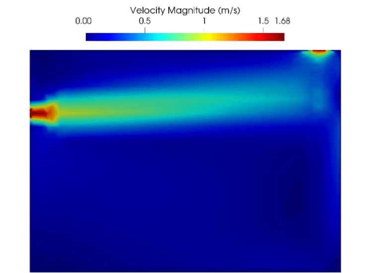
Figure 2: velocity profile in the x-z plane at y=1.8 m.
Furthermore, the MAA in the same plane for which the velocity profile was depicted in Figure 2 is represented in.
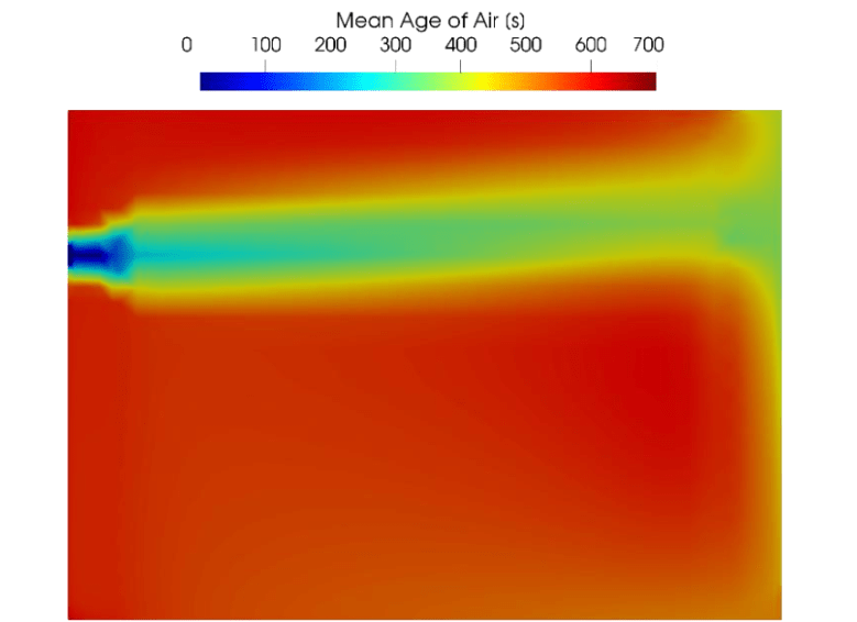
Figure 3: MAA profile in the x-z plane at y=1.8 m
The MAA shown in this figure owns the units of sec. On the other hand, as mentioned in the previous section, we need to calculate the dimensionless form of MAA in order to properly compare the experimental and CFD results. In order to confirm the validity of the solutions, as mentioned above, the dimensionless MAA was calculated based on the flow field found by solving equation 1 using SST 𝑘 – 𝜔 method. The dimensionless MAA for three different locations shown in Figure 1 are depicted in Figure 4(a)-(c). One may note that since the numerical points were not coinciding with the locations of measured points, the lines in the figures are obtained after bilinear interpolation.
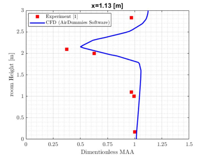
Figure 4 (a): Dimensionless MAA at different room heights at the location of x=1.13m from the west wall
towards the east wall. It is worth mentioning that this point is located in the middle plane, i.e., at y=1.8m.
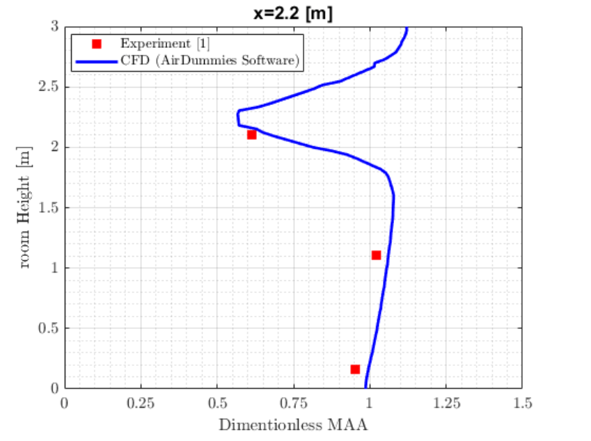
Figure 4 (b): Dimensionless MAA at different room heights at the location of x=2.2m from the west wall
towards the east wall. It is worth mentioning that this point is located in the middle plane, i.e., at y=1.8m.
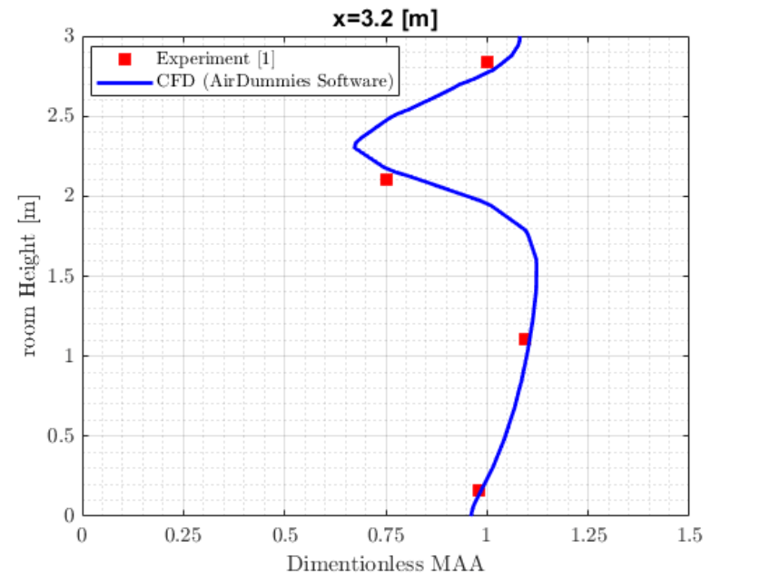
Figure 4 (c): Dimensionless MAA at different room heights at the location of x=3.2m from the west wall
towards the east wall. It is worth mentioning that this point is located in the middle plane, i.e., at y=1.8m.
Looking at the results from figure 4(a)-(c), one can make the following conclusions:
- MAA distribution follows the airflow patterns in the room increasing gradually from the inlet along the jet and reaching the highest values in recirculation zones with stagnant air.
- There experimental results obtained by [reference] are similar to the ones given by the AirDummies CFD tool.
- Although the grid points are not exactly at the same points where the MAA was calculated experimentally, the results still agree very well even at the height of 2 m which is close to the air inlet where the velocity field has the highest gradient.
- Use of (SST) 𝑘 – 𝜔 shows great promise in solving air flows in room air ventilation problems both close to the wall and in the far field zone.
- The dimensionless MAA was used which shows that the validation holds true for all other room dimensions with various air flow rates.
Conclusion
The current work represented the mean age of air at three different spots in a room ventilated with fresh air at constant temperature.
The results were obtained using the AirDummies CFD software package. The main goal of this research has been to compare the results obtained by AirDummies with the real experimental data. Dimensionless form of MAA was used to generalize the validation to all room dimensions and all air flow rates. The results showed that the numerical solution solves the flow field equation both close to the walls and in the far field regions, thanks to use of robust and efficient method of (SST) 𝑘 – 𝜔.
References
- Bartak, M., et al., Experimental and numerical study of local mean age of air.2001.
- Menter, F.R., Two-equation eddy viscosity turbulence models for engineering applications. AIAA journal, 1994. 32(8): p. 1598-1605.
- Denev, J.A., F. Durst, and B. Mohr, Room ventilation and its influence on the performance of fume cupboards: a parametric numerical study. Industrial & engineering chemistry research, 1997. 36(2): p. 458-466.
- Stankov, P., J. Denev, and Y. Dinkov. Three dimensional room airflow: computation and estimation of the ventilation efficiency. in the proc. International Symposium Air Flow in Multizone Structures (Budapest). 1992.
Here is downloadable file: Btec-Validation-Final Version2